Tracking the Spin on a Ping Pong Ball
with the Quaternion Bingham Filter
Jared Glover and Leslie Pack Kaelbling
Abstract— A deterministic method for sequential estimation
of 3-D rotations is presented. The Bingham distribution is
used to represent uncertainty directly on the unit quaternion
hypersphere. Quaternions avoid the degeneracies of other 3-D
orientation representations, while the Bingham distribution
allows tracking of large-error (high-entropy) rotational dis-
tributions. Experimental comparison to a leading EKF-based
filtering approach on both synthetic signals and a ball-tracking
dataset shows that the Quaternion Bingham Filter (QBF) has
lower tracking error than the EKF, particularly when the
state is highly dynamic. We present two versions of the QBF–
suitable for tracking the state of first- and second-order rotating
dynamical systems.
I. INTRODUCTION
As any fan of this high-speed sport knows, table tennis
is a game of spin. Because of the high-friction soft rubber
surfaces of modern ping pong paddles, ball spin—which can
reach 150 rotations per second—plays an enormous role in
determining the trajectory of the ball after being hit. A top-
spin ball tends to fly off of your paddle up into the air, while
an under-spin ball will drop down into the net. Due to air
resistance, spin can also change the in-flight trajectories of
balls as well, a phenomenon known as the “Magnus effect”
which leads to the well-known “curveball” in the sport of
baseball. Ping pong players go to great length to disguise
the spins they put on the ball, and much of the training of
table tennis professionals goes into the technique and strategy
of handling different types of spins. Swings which impart
different types of spin are given different names, like “loop”,
“chop”, “push”, and “flip”.
Several robots have been programmed to play ping pong
over the years [1], [16], [20], [17]. However, only the earliest
of these systems (by Russell Andersson in the late 1980s)
made any attempt to track the spin on the ball. Because
it used only indirect measurements of the spin (via the
Magnus effect), the spin estimates were extremely noisy [1].
Fortunately for Andersson, he used only low-friction wooden
paddles (with no rubber surface), so the effects of spin were
minimized, and the robot was able to hold its own against
novice players at moderate speeds and spins.
In this paper we present an approach to track the spin on
the ping pong ball from direct measurements of the ball’s
This work was supported in part by the NSF under Grant No. 1117325.
Any opinions, findings, and conclusions or recommendations expressed in
this material are those of the author(s) and do not necessarily reflect the
views of the National Science Foundation. We also gratefully acknowledge
support from ONR MURI grant N00014-09-1-1051, from AFOSR grant
FA2386-10-1-4135 and from the Singapore Ministry of Education under a
grant to the Singapore-MIT International Design Center.
Jared Glover and Leslie Pack Kaelbling are with the Massachusetts
Institute of Technology. Email: {jglov,lpk}@mit.edu
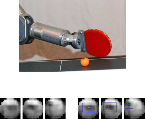
Fig. 1. Our ping pong robot uses a 7-dof Barrett WAM arm with a ping
pong paddle rigidly attached at the wrist.
Fig. 2. Detecting the logo on a ping pong ball in high-speed images can
be a tricky task, due to the small size of the ball (40mm) and the motion
blur. (Left) Original images. (Right) Ball orientation estimates.
orientation with a high-speed camera (Figure 2).
3-D rotational data occurs in many disciplines, from geol-
ogy to robotics to physics. Yet modern statistical inference
techniques are seldom applied to such data sets, due to
the complex topology of 3-D rotation space, and the well-
known aliasing problems caused by orientations “wrapping
around” back to zero. Many probability distributions exist
for modeling uncertainty on rotational data, yet difficulties
often arise in the mechanics of complex inference tasks.
The technical contribution of this paper is to explore one
distribution—the Bingham—which is particularly well-suited
for inference, and to derive some common operations on
Bingham distributions as a reference for future researchers.
We present a new deterministic method—the Quaternion
Bingham Filter (QBF)—for approximate recursive inference
in quaternion Bingham processes. The quaternion Bingham
process is a type of dynamic Bayesian network (DBN)
on 3-D rotational data, where both process dynamics and
measurements are perturbed by random Bingham rotations.
The QBF uses the Bingham distribution to represent state
uncertainty on the unit quaternion hypersphere. Quaternions
avoid the degeneracies of other 3-D orientation represen-
tations, while the Bingham enables accurate tracking of
high-noise signals. Performing exact inference on quaternion
Bingham processes requires the composition of Bingham
distributions, which results in a non-Bingham density. There-
fore, we approximate the resulting composed distribution as

a Bingham using the method of moments, in order to keep
the filtered state distribution in the Bingham family.
We compare the quaternion Bingham filter to a previous
approach to tracking rotations based on the Extended Kalman
Filter (EKF) and find that the QBF has lower tracking
error than the EKF, particularly when the state is highly
dynamic. We evaluate the performance of the QBF on both
synthetic rotational process signals and on a real dataset
containing 3-D orientation estimates of a spinning ping-pong
ball tracked in high-speed video. We also derive the true
probability density function (PDF) for the composition of
two Bingham distributions, and report the empirical error of
the moment-matching composition approximation for various
distributions. We begin by introducing the Bingham distribu-
tion and presenting operations on it that will be needed by the
filter. Then, we derive the first- and second-order quaternion
Bingham processes and the QBF for estimating their state.
We conclude with experiments on artificial and real data.
II. DISTRIBUTIONS ON ROTATIONS
The problem of how to represent a probability distribution
on the space of rotations in three dimensions has been a
subject of considerable study. Representing the distribution
directly in the space of Euler angles is difficult because
of singularities in the space when two of the angles are
aligned (known as gimbal lock). A more appropriate space
for representing distributions on rotations is the space of unit
quaternions: a rotation becomes a point on the 4-dimensional
unit hypersphere, S
3
. This space lacks singularities, but has
the difficulty that the representation is not unique: both q
and −q represent the same rotation. Putting a Gaussian
distribution directly in quaternion space does not respect
the underlying topology of 3-D rotations; however, this
approach has been the basis of tracking methods based on
approximations of the Kalman filter [13], [4], [15], [5], [10],
[11]. A more appropriate method is to represent distributions
in an R
3
space that is tangent to the quaternion hypersphere
at the mean of the distribution [6]; but such a tangent-space
approach will be unable to effectively represent distributions
that have large variances. In many perceptual problems, it
may be possible to make observations that provide significant
information about only one or two dimensions, yielding high-
variance estimates. For this reason, we use the Bingham
distribution.
The Bingham distribution is commonly used as a distri-
bution on 3-D rotations as unit quaternions [2], [9], [18]. Its
density function (PDF) is given by
f(x; Λ, V ) =
1
F
exp{
d
X
i=1
λ
i
(v
i
T
x)
2
} (1)
where x is a unit vector on the surface of the sphere S
d
⊂
R
d+1
, F is a normalization constant, Λ is a vector of non-
positive (≤ 0) concentration parameters, and the columns v
i
of the (d + 1) × d matrix V are orthogonal unit vectors.
The Bingham distribution is the maximum entropy distri-
bution on the hypersphere which matches the sample inertia
matrix E[xx
T
] [14]. Therefore, it may be better suited
to representing random process noise on the hypersphere
than some other distributions, such as (projected) tangent-
space Gaussians. Binghams are also quite flexible, since
a concentration parameter, λ
i
, of zero indicates that the
distribution is completely uniform in the direction of v
i
.
They are therefore very useful in tracking problems where
there is high, anisotropic noise. For example, to track the
ping pong ball based on detections of its logo, the position
of the logo can often be detected much more reliably than
its orientation, so the axis (from the center of the ball to the
logo) of the ball’s 3-D orientation estimate will have less
uncertainty than the angle.
III. OPERATIONS ON BINGHAM DISTRIBUTIONS
In order to implement the quaternion Bingham filter, we
need to be able to perform several operations on Bingham
distributions. To our knowledge, all of these operations,
except for computing the normalization constant, are new
contributions of this paper. More operations (including cal-
culation of KL-divergence and sampling methods) are pre-
sented in the accompanying tech report [7].
The Normalization constant. The primary difficulty with
using the Bingham distribution in practice lies in computing
the normalization constant, F . Since the distribution must
integrate to one over its domain (S
d
), we can write the
normalization constant as
F (Λ) =
Z
x∈S
d
exp{
d
X
i=1
λ
i
(v
i
T
x)
2
} = |S
d
|·
1
F
1
(
1
2
;
d + 1
2
; Λ)
(2)
where
1
F
1
() is a hyper-geometric function of matrix argu-
ment [2]. Evaluating
1
F
1
() is expensive, so we precompute
a lookup table of F -values over a discrete grid of Λ’s, and
use tri-linear interpolation to quickly estimate normalizing
constants on the fly.
Product of Bingham PDFs. The correction step of the fil-
ter requires multiplying PDFs. The product of two Bingham
PDFs is given by adding their exponents:
f(x;Λ
1
, V
1
)f(x; Λ
2
, V
2
)
=
1
F
1
F
2
exp{x
T
(
d
X
i=1
λ
1i
v
1i
v
1i
T
+ λ
2i
v
2i
v
2i
T
)x}
=
1
F
1
F
2
exp{x
T
(C
1
+ C
2
)x}
(3)
After computing the sum C = C
1
+ C
2
in the exponent
of equation 3, we transform the PDF to standard form by
computing the eigenvectors and eigenvalues of C, and then
subtracting off the lowest magnitude eigenvalue from each
spectral component, so that only the eigenvectors corre-
sponding to the largest d eigenvalues (in magnitude) are kept,
and λ
1
≤ · · · ≤ λ
d
≤ 0 (as in equation 1).
Rotation by a fixed quaternion. To find the effect of the
control on the predictive distribution, we rotate the prior by
u. Given q ∼ Bingham(Λ, V ), u ∈ S
3
, and s = u ◦ q,
then s ∼ Bingham(Λ, u ◦ V ), where u ◦ V , [u ◦ v
1
, u ◦
v
2
, u ◦ v
3
]. In other words, s is distributed according to
a Bingham whose orthogonal direction vectors have been
rotated (on the left) by u. Similarly, if s = q ◦ u then s ∼
Bingham(Λ, V ◦ u).
Proof for s = u ◦ q: Since unit quaternion rotation is
invertible and volume-preserving, we have
f
s
(s) = f
q
(u
−1
◦ s) =
1
F
exp{
d
X
i=1
λ
i
(v
i
T
(u
−1
◦ s))
2
}
=
1
F
exp{
d
X
i=1
λ
i
((u ◦ v
i
)
T
s)
2
} .
Quaternion inversion. Given q ∼ Bingham(Λ, V ) and
s = q
−1
, then s ∼ Bingham( Λ , JV ), where J is the
quaternion inversion matrix, J =
1
−1
−1
−1
. The proof
follows the same logic as in the previous section.
Composition of quaternion Binghams. Implementing the
QBF requires the computation of the PDF of the composition
of two independent Bingham random variables. Letting q ∼
Bingham(Λ, V ) and r ∼ Bingham(Σ, W ), we wish to find
the PDF of s = q ◦ r.
The true distribution is the convolution, in S
3
, of the
PDFs of the component distributions
1
.
f
true
(s) =
Z
q∈S
3
f(s|q)f(q)
=
1
F
1
(
1
2
;
4
2
; C(s))
|S
3
| ·
1
F
1
(
1
2
;
4
2
; Λ)
1
F
1
(
1
2
;
4
2
; Σ)
, (4)
where C(s) =
P
3
i=1
σ
i
(s ◦ w
i
−1
)(s ◦ w
i
−1
)
T
+ λ
i
v
i
v
i
T
.
To approximate the PDF of s with a Bingham density,
f
B
(s) = f
B
(q ◦ r), it is sufficient to compute the second
moments of q ◦ r, since the inertia matrix, E[ss
T
] is the
sufficient statistic for the Bingham. This moment-matching
approach is equivalent to the variational approach, where f
B
is found by minimizing the KL divergence from f
B
to f
true
.
Noting that q ◦ r can be written as
(q
T
H
T
1
r, q
T
H
T
2
r, q
T
H
T
3
r, q
T
H
T
4
r), where
H
1
=
1 0 0 0
0 1 0 0
0 0 1 0
0 0 0 1
, H
2
=
0 −1 0 0
1 0 0 0
0 0 0 1
0 0 −1 0
, H
3
=
0 0 −1 0
0 0 0 −1
1 0 0 0
0 1 0 0
,
and H
4
=
0 0 0 −1
0 0 1 0
0 −1 0 0
1 0 0 0
, we find that
E[s
i
s
j
] = E[q
T
H
T
i
rr
T
H
j
q] ,
which has 16 terms of the form ±r
a
r
b
q
c
q
d
, where a, b, c, d ∈
{1, 2, 3, 4}. Since q and r are independent, E[±r
a
r
b
q
c
q
d
] =
±E[r
a
r
b
]E[q
c
q
d
]. Therefore (by linearity of expectation),
every entry in the matrix E[ss
T
] is a quadratic function of
elements of the inertia matrices of q and r, which can be
easily computed given the Bingham normalization constants
and their partial derivatives. The entire closed form for
E[ss
T
] is given in the accompanying tech report [7].
Estimating the error of approximation. To estimate the
error in the Bingham approximation to the composition of
1
See the accompanying tech report for a full derivation [7].
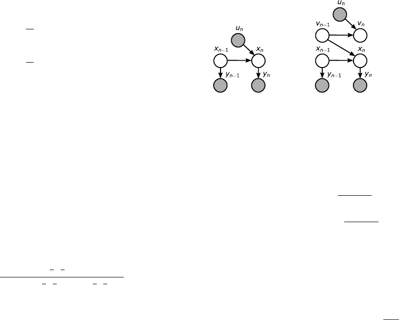
First-order
x
n
= w
n
◦ u
n
◦ x
n−1
y
n
= z
n
◦ x
n
Second-order
v
n
= w
n
◦ u
n
◦ v
n−1
x
n
= v
n−1
◦ x
n−1
y
n
= z
n
◦ x
n
Fig. 3. Process and graphical models for the discrete quaternion Bingham
process.
two quaternion Bingham distributions, B
1
◦ B
2
, we approx-
imate the KL divergence from f
B
to f
true
using a finite
element approximation on the quaternion hypersphere
D
KL
(f
B
k f
true
) =
Z
x∈S
3
f
B
(x) log
f
B
(x)
f
true
(x)
≈
X
x∈F(S
3
)
f
B
(x) log
f
B
(x)
f
true
(x)
· ∆x
where F(S
d
) and {∆x} are the points and volumes of the
finite-element approximation to S
3
, based on a recursive
tetrahedral-octahedral subdivision method [19].
Entropy. The entropy of a Bingham distribution with PDF
f is given by:
h(f) = −
Z
x∈S
d
f(x) log f(x) = log F − Λ ·
∇F
F
.
(5)
The proof is given in the accompanying tech report [7]. Since
both the normalization constant, F , and its gradient with
respect to Λ, ∇F , are stored in a lookup table, the entropy
is trivial to approximate via interpolation, and can be used on
the fly without any numerical integration over hyperspheres.
IV. DISCRETE-TIME QUATERNION BINGHAM PROCESS
The first-order discrete-time quaternion Bingham process
has, as its state, x
n
, a unit quaternion representing the
orientation of interest at time n. The system’s behavior
is conditioned on control inputs u
n
, which are also unit
quaternions. The new orientation is the old orientation rotated
by the control input and then by independent noise w
n
∼
Bingham(Λ
p
, V
p
). Note that “◦” denotes quaternion multi-
plication, which corresponds to composition of rotations for
unit quaternions. (q ◦ r means “rotate by r and then by q”.)
The second-order quaternion Bingham process has state
(x
n
, v
n
), where x
n
represents orientation and the quaternion
v
n
represents discrete rotational velocity at time n. The
control inputs u
n
are analogous to rotational accelerations.
Process noise w
n
enters the system in the velocity dynamics.
In both the first-order and second-order systems, obser-
vations y
n
are given by the orientation x
n
corrupted by
independent Bingham noise z
n
∼ Bingham(Λ
o
, V
o
). One

common choice for V
p
and V
o
is
0 0 0
1 0 0
0 1 0
0 0 1
, which means
that the mode is the quaternion identity, (1, 0, 0, 0). (Any
V matrix whose top row contains all zeros will have this
mode.) Figure 3 shows the process and graphical models for
the discrete quaternion Bingham process.
V. DISCRETE QUATERNION BINGHAM FILTER
The state of a discrete-time quaternion Bingham process
can be estimated using a discrete-time quaternion Bingham
filter, which is a recursive estimator similar in structure to a
Kalman filter. Unlike the Kalman filter, however, the QBF is
approximate, in the sense that the tracked state distribution
is projected to be in the Bingham family after every time
step. The second-order QBF will also require an assumption
of independence between x
n
and v
n
, given all the data
up to time n. Both the first-order and second-order QBFs
are examples of assumed density filtering—a well-supported
approximate inference method in the DBN literature [3]. We
will start by deriving the first-order QBF, which follows
the Kalman filter derivation quite closely. Note that the
following derivations rely on several properties of Bingham
distributions which were detailed in section III.
First-order QBF. Given a distribution over the initial state
x
0
, B
x
0
∼ Bingham(Λ
0
, V
0
), and an action-observation
sequence u
1
, y
1
, . . . , u
n
, y
n
, the goal is to compute the
posterior distribution f(x
n
| u
1
, y
1
, . . . , u
n
, y
n
). We can
use Bayes’ rule and the Markov property to decompose this
distribution as follows:
B
x
n
= f(x
n
|u
1
, y
1
, . . . , u
n
, y
n
)
∝ f(y
n
|x
n
)f(x
n
|u
1
, y
1
, . . . , u
n−1
, y
n−1
, u
n
)
= f(y
n
|x
n
)
Z
x
n−1
f(x
n
| x
n−1
, u
n
)B
x
n−1
(x
n−1
)
= f(y
n
|x
n
)(f
w
n
◦ u
n
◦ B
x
n−1
)(x
n
) .
where f
w
n
◦ u
n
◦ B
x
n−1
means rotate B
x
n−1
by u
n
and
then convolve with the process noise distribution, f
w
n
. For
the first term, f (y
n
|x
n
), recall that the observation process
is y
n
= z
n
◦ x
n
, so y
n
|x
n
∼ Bingham(y
n
; Λ
o
, V
o
◦ x
n
),
where we used the result from section III for rotation of
a Bingham by a fixed quaternion. Thus the distribution for
y
n
|x
n
is
f(y
n
|x
n
) =
1
F
o
exp
3
X
i=1
λ
oi
(y
n
T
(v
oi
◦ x
n
))
2
.
Now we can rewrite y
n
T
(v
oi
◦ x
n
) as (v
−1
oi
◦ y
n
)
T
x
n
,
so that f(y
n
|x
n
) is a Bingham density on x
n
,
Bingham(x
n
; Λ
o
, V
−1
o
◦ y
n
). Thus, computing B
x
n
reduces to multiplying two Bingham PDFs on x
n
, which is
given in section III.
Second-order QBF. Given a factorized distribution
over the initial state f(x
0
, v
0
) = B
x
0
B
v
0
and an
action-observation sequence u
1
, y
1
, . . . , u
n
, y
n
, the goal
is to compute the joint posterior distribution f(x
n
, v
n
|
u
1
, y
1
, . . . , u
n
, y
n
). However, the joint distribution on x
n
and v
n
is too difficult to represent, so we instead compute
the marginal posteriors over x
n
and v
n
separately, and ap-
proximate the joint posterior as the product of the marginals.
The marginal posterior on x
n
is
B
x
n
= f(x
n
|u
1
, y
1
, . . . , u
n
, y
n
)
∝ f(y
n
|x
n
)
Z
x
n−1
f(x
n
|x
n−1
)B
x
n−1
(x
n−1
)
= f(y
n
|x
n
)(B
v
n−1
◦ B
x
n−1
)(x
n
)
since we assume x
n−1
and v
n−1
are independent given all
the data up to time n − 1.
Similarly, the marginal posterior on v
n
is
B
v
n
= f(v
n
|u
1
, y
1
, . . . , u
n
, y
n
)
∝
Z
v
n−1
f(v
n
| v
n−1
, u
n
)B
v
n−1
(v
n−1
)
·
Z
x
n
f(y
n
|x
n
)f(x
n
|v
n−1
, u
1
, y
1
, . . . , u
n−1
, y
n−1
).
Once again, f(y
n
|x
n
) can be written as a Bingham density
on x
n
, Bingham(x
n
; Λ
o
, V
−1
o
◦ y
n
). Next, note that x
n
=
v
n−1
◦ x
n−1
so that f(x
n
|v
n−1
, u
1
, y
1
, . . . , u
n−1
, y
n−1
) =
B
x
n−1
(v
−1
n−1
◦ x
n
), which can also be re-written as a Bing-
ham on x
n
. Now letting x
n−1
∼ Bingham(Σ, W ), and since
the product of two Bingham PDFs is Bingham, the integral
over x
n
becomes proportional to a Bingham normalization
constant,
1
F
1
(
1
2
;
4
2
; C(v
n−1
)), where
C(v
n−1
) =
3
X
i=1
σ
i
(v
n−1
◦ w
i
)(v
n−1
◦ w
i
)
T
+ λ
oi
(v
−1
oi
◦ y
n
)(v
−1
oi
◦ y
n
)
T
.
Comparing C(v
n−1
) with equation 4 in section III we find
that
1
F
1
(
1
2
;
4
2
; C(v
n−1
)) ∝ (f
y
n
|x
n
◦ B
−1
x
n−1
)(v
n−1
). Thus,
B
v
n
∝
Z
v
n−1
f(v
n
| v
n−1
, u
n
)B
v
n−1
(v
n−1
)
· (f
y
n
|x
n
◦ B
−1
x
n−1
)(v
n−1
)
= (f
w
n
◦ u
n
◦ (B
v
n−1
· (f
y
n
|x
n
◦ B
−1
x
n−1
)))(v
n
)
In other words, to update the belief on v
n
, we first
convolve the inverse belief on x
n−1
with the measurement
distribution, then multiply by the belief on v
n−1
, rotate by
the control input u
n
, and convolve by the noise distribu-
tion, f
w
n
. In the next section, each of these operations on
Bingham distributions will be explained in detail.
A. Extensions
For some applications (such as tracking a ping pong ball
through a bounce), the process and observation models of the
QBFs described above may be somewhat restrictive. Several
extensions are possible, as we outline here.
Sampling-based methods / Tracking the ball through a
bounce. The QBF can handle arbitrary process and control
models by sampling from the current state distribution,
applying the process/control function to each sample, and
then fitting new Bingham distributions to the resulting post-
process/control samples. This is precisely the method we use
in our experiments to track the ping pong ball through a
bounce on the table. The process model is taken from Ander-
sson’s ball physics derivation [1], and is a complex function
of the ball’s tracked angular and translational velocities,
w
f
= w
i
+
3µ
2r
(ˆv
ry
, −ˆv
rx
, 0)v
iz
(1 + ǫ),
where w
i
and w
f
are the initial and final (pre- and post-
bounce) angular velocity vectors, µ and ǫ are the coefficients
of friction and restitution, r is the ball’s radius, v
iz
is the
ball’s initial translational z-velocity, and ˆv
r
= v
r
/kv
r
k,
where v
r
= (v
iy
+w
ix
r, v
ix
−w
iy
r, 0) is the relative velocity
of the surface of the ball with respect to the table.
Quaternion exponentiation / Continuous-time filters.
Quaternion exponentiation for unit quaternions is akin to
scaling in Euclidean space. If q represents a 3-D rotation
of angle θ about the axis v, then q
a
is a rotation of aθ about
v. This operation would be needed to handle a continuous-
time update in the second-order Bingham filter, since the
orientation needs to be rotated by some fraction of the spin
quaternion at each (time-varying) time step.
It is possible to incorporate quaternion exponentiation
in all parts of the model via a moment-matching method
for Bingham exponentiation (akin to the moment-matching
method for Bingam composition). However, an additional
Taylor-approximation is needed to approximate the second
moments of the exponentiated Bingham as a function of the
second and higher even moments of the original distribution.
(The odd moments of a Bingham are always zero due to
symmetry.)
VI. EXPERIMENTAL RESULTS
We compare the quaternion Bingham filter against an
extended Kalman filter (EKF) approach in quaternion
space [13], where process and observation noise are gen-
erated by Gaussians in R
4
, the measurement function nor-
malizes the quaternion state (to project it onto the unit
hypersphere), and the state estimate is renormalized after
every update. We chose the EKF both due to its popularity
and because LaViola reports in [13] that it has similar
(slightly better) accuracy to the unscented Kalman filter
(UKF) in several real tracking experiments. We adapted
two versions of the EKF (for first-order and second-order
systems) from LaViola’s EKF implementation by changing
from a continuous to a discrete time prediction update.
We also mapped QBF (Bingham) noise parameters to EKF
(Gaussian) noise parameters by empirically matching second
moments from the Bingham to the projected Gaussian—
i.e., the Gaussian after it has been projected onto the unit
hypersphere.
Synthetic Data. To test the first-order quaternion
Bingham filter, we generated several synthetic signals
by simulating a quaternion Bingham process, where the
(velocity) controls were generated so that the nominal
process state (before noise) would follow a sine wave
pattern on each angle in Euler angle space. We chose this
control pattern in order to cover a large area of 3-D rotation
space with varying rotational velocities. Two examples of
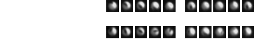
(a) slow top-spin (b) fast top-spin
(c) slow side-spin (d) fast side-spin
Fig. 5. Example image sequences from the spinning ping-pong ball
dataset. In addition to lighting variations and low image resolution, high
spin rates make this dataset extremely challenging for orientation tracking
algorithms. Also, because the cameras were facing top-down towards the
table, tracking side-spin relies on correctly estimating the orientation of the
elliptical marking in the image, and is therefore much harder than tracking
top-spin or under-spin.
synthetic signals along with quaternion Bingham filter output
are shown in figure 4. Their observation parameters were
Λ
o
= (−50, −50, −50), which gives moderate, isotropic
observation noise, and Λ
o
= (−10, −10, −1), which yields
moderately high noise in the first two directions, and
near-uniform noise in the third direction. We estimated
the composition approximation error (KL-divergence) for
9 of these signals, with both isotropic and nonisotropic
noise models, from all combinations of (Λ
p
, Λ
o
) in
{(−50, −50, −50), (−200, −200, −200), (−10, −10, −1)}.
The mean composition error was .0012, while the max
was .0197, which occurred when Λ
p
and Λ
o
were both
(−10, −10, −1).
For the EKF comparison, we wanted to give the EKF the
best chance to succeed, so we generated the data from a
projected Gaussian process, with process and observation
noise generated according to a projected Gaussian (in or-
der to match the EKF dynamics model) rather than from
Bingham distributions. We ran the first-order QBF and EKF
on 270 synthetic projected Gaussian process signals (each
with 1000 time steps) with different amounts of process and
observation noise, and found the QBF to be more accurate
than the EKF on 268/270 trials. The mean angular change in
3-D orientation between time steps were 7, 9, and 18 degrees
for process noise parameters -400, -200, and -50, respectively
(where -400 means Λ
p
= (−400, −400 − 400), etc.).
The most extreme cases involved anisotropic observation
noise, with an average improvement over the EKF mean error
rate of 40-50%. The combination of high process noise and
low observation noise also causes trouble for the EKF. Table I
summarizes the results.
Spinning ping-pong ball dataset To test the second-
order QBF, we collected a dataset of high-speed videos of
73 spinning ping-pong balls in flight (Figure 5). On each
ball we drew a solid black ellipse over the ball’s logo to
allow the high-speed (200fps) vision system to estimate the
ball’s orientation by finding the position and orientation
of the logo
2
. However, an ellipse was only drawn on one
side of each ball, so the ball’s orientation could only be
estimated when the logo was visible in the image. Also, since
ellipses are symmetric, each logo detection has two possible
2
Detecting the actual logo on the ball, without darkening it with a marker,
would require improvements to our camera setup.
0 20 40 60 80 100 120 140 160 180 200
−1
−0.5
0
0.5
1
qw
0 20 40 60 80 100 120 140 160 180 200
−1
−0.5
0
0.5
1
qx
0 20 40 60 80 100 120 140 160 180 200
−1
−0.5
0
0.5
1
qy
0 20 40 60 80 100 120 140 160 180 200
−1
−0.5
0
0.5
1
qz
0 20 40 60 80 100 120 140 160 180 200
0
0.1
0.2
0.3
0.4
error
(a) Λ
o
= (−50, −50, −50)
0 20 40 60 80 100 120 140 160 180 200
−1
−0.5
0
0.5
1
qw
0 20 40 60 80 100 120 140 160 180 200
−1
−0.5
0
0.5
1
qx
0 20 40 60 80 100 120 140 160 180 200
−1
−0.5
0
0.5
1
qy
0 20 40 60 80 100 120 140 160 180 200
−1
−0.5
0
0.5
1
qz
0 20 40 60 80 100 120 140 160 180 200
0
0.5
1
1.5
2
error
(b) Λ
o
= (−10, −10, −1)
0 20 40 60 80 100 120 140 160 180 200
−1
−0.5
0
0.5
1
qw
0 20 40 60 80 100 120 140 160 180 200
−1
−0.5
0
0.5
1
qx
0 20 40 60 80 100 120 140 160 180 200
−1
−0.5
0
0.5
1
qy
0 20 40 60 80 100 120 140 160 180 200
−1
−0.5
0
0.5
1
qz
(c) Λ
o
= (−10, −10, −1)
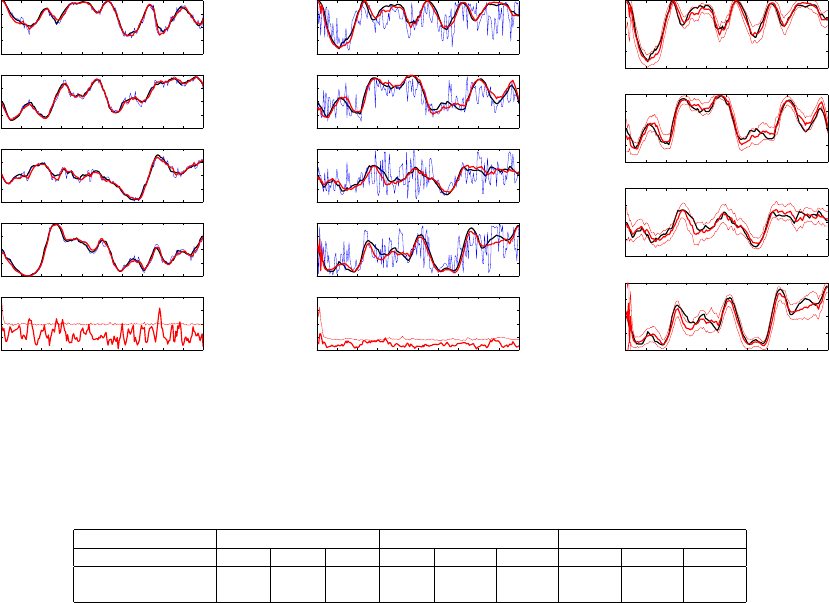
Fig. 4. Two simulated runs with the quaternion Bingham filter—(b) and (c) are different plots of the same simulation. In all figures, the thick black line
is the true process signal, generated with isotropic process noise Λ
p
= (−400, −400, −400). The thin blue lines in (a) and (b) are the observation signal,
and the thick red line is the filtered output. Rows 1-4 in each figure show the 4 quaternion dimensions (q
w
, q
x
, q
y
, q
z
). Row 5 in (a) and (b) shows the
error between filter output and true state (thick red line), together with the QBF sample error 90% confidence bounds (thin red line). Marginal sample 90%
confidence bounds are also shown in the thin red lines in (c).
observation noise -400, -400, -10 -400 -50
process noise -50 -200 -400 -50 -200 -400 -50 -200 -400
% improvement 37.3 45.6 54.3 19.9 3.33 1.52 3.42 0.72 0.47
± (5.1) (5.0) (6.4) (1.8) (0.53) (0.44) (0.88) (0.40) (0.27)
TABLE I
PROJECTED GAUSSIAN PROCESS SIMULATIONS. AVERAGE % MEAN ERROR DECREASE FOR QBF OVER EKF.
orientation interpretations
3
. The balls were spinning at 25-
50 revolutions per second (which equates to a 45-90 degree
orientation change per frame), making the filtering problem
extremely challenging due to aliasing effects. We used a ball
gun to shoot the balls with consistent spin and speed, at 4
different spin settings (topspin, underspin, left-sidespin, and
right-sidespin) and 3 different speed settings (slow, medium,
fast), for a total of 12 different spin types. Although we
initially collected videos of 107 ball trajectories, the logo
could only be reliably found in 73 of them; the remaining
34 videos were discarded. Although not our current focus,
adding more cameras, adding markings to the ball, and
improving logo detections would allow the ball’s orientation
and spin to be tracked on a larger percentage of such videos.
To establish an estimate of ground truth, we then manually
labeled each ball image with the position and orientation
of the logo (when visible), from which we recovered the
ball orientation (up to symmetry). We then used least-squares
non-linear regression to smooth out our (noisy) manual labels
by finding the constant rotation,
ˆ
s, which best fit the labeled
orientations for each trajectory
4
.
3
We disambiguated between the two possible ball orientation observations
by picking the observation with highest likelihood under the current QBF
belief.
4
Due to air resistance and random perturbations, the spin was not really
constant throughout each trajectory. But for the short duration of our
experiments (40 frames), the constant spin approximation was sufficient.
To run the second-order QBF on this data, we initialized
the QBF with a uniform orientation distribution B
x
0
and
a low concentration (Λ = (−3, −3 − 3)) spin distribution
B
v
0
centered on the identity rotation, (1, 0, 0, 0). In other
words, we provided no information about the ball’s initial
orientation, and an extremely weak bias towards slower
spins. We also treated the “no-logo-found” (a.k.a. “dark
side”) observations as a very noisy observation of the logo
in the center of the back side of the ball at an arbitrary
orientation, with Λ
o
= (−3.6, −3.6, 0)
5
. When the logo was
detected, we used Λ
o
= (−40, −40, −10) for the observation
noise. A process noise with Λ
p
= (−400, −400, −400) was
used throughout, to account for small perturbations to spin.
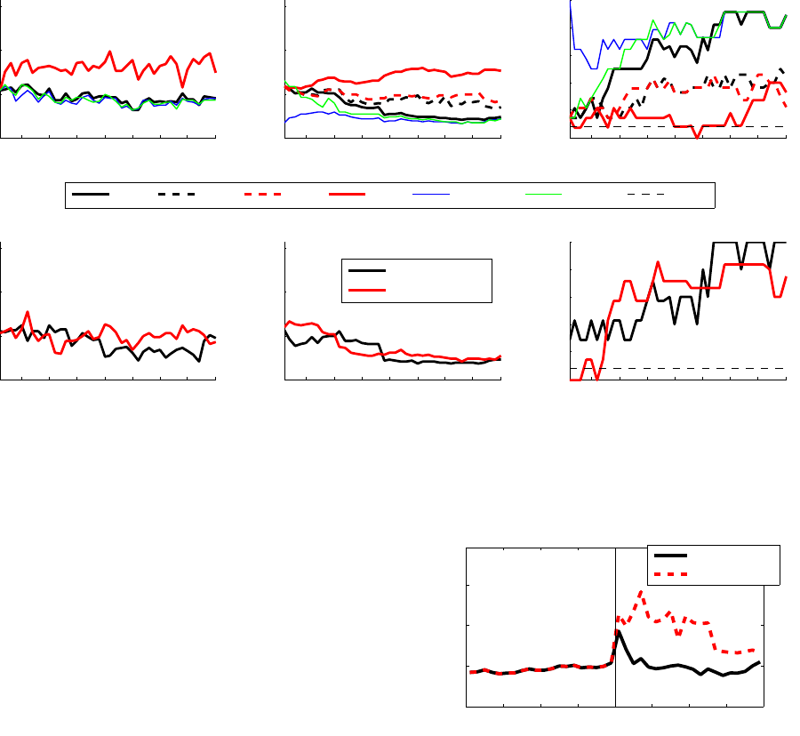
Results of running the second-order QBF (QBF-2) are
shown in figure 6. We compared the second-order QBF
to the second-order EKF (EKF-2) and also to the first-
order QBF and EKF (QBF-1 and EKF-1), which were given
the difference between subsequent orientation observations
as their observations of spin. The solid, thin, blue line
in each plot marked “oracle prior” shows results from
running QBF-2 with a best-case-scenario prior, centered
on the average ground truth spin for that spin type, with
Λ = (−10, −10, −10). We show mean orientation and spin
errors (to regressed ground truth), and also spin classification
accuracy using the MAP estimate of spin type (out of 12)
5
We got this Λ
o
by fitting a Bingham to all possible dark side orientations.
5 10 15 20 25 30 35 40
0
0.5
1
1.5
orientation error
radians
time
5 10 15 20 25 30 35 40
0
0.5
1
1.5
spin error
radians
time
5 10 15 20 25 30 35 40
0
0.2
0.4
0.6
0.8
1
spin classification
accuracy
time
QBF−2
QBF−1 EKF−1 EKF−2 oracle prior filter bank random
5 10 15 20 25 30 35 40
0
0.5
1
1.5
orientation error
radians
time
5 10 15 20 25 30 35 40
0
0.5
1
1.5
spin error
radians
time
5 10 15 20 25 30 35 40
0
0.2
0.4
0.6
0.8
1
spin classification
accuracy
time
topspin/underspin
sidespin
Fig. 6. Spinning ping-pong ball tracking results. Top row: comparison of QBF-2 (with and without an oracle-given prior) to QBF-1, EKF-1, EKF-2,
and random guessing (for spin classification); QBF-1 and EKF-1 do not show up in the orientation error graph because they only tracked spin. Note that
QBF-2 quickly converges to the oracle error and classification rates. Bottom row: QBF-2 results broken down into top-spin/under-spin vs. side-spin. As
mentioned earlier, the side-spin data is harder to track due to the chosen camera placement and ball markings for this experiment.
given the current spin belief
6
. The results clearly show that
QBF-2 does the best job of identifying and tracking the ball
rotations on this extremely challenging dataset, achieving a
classification rate of 91% after just 30 video frames, and a
mean spin (quaternion) error of 0.17 radians (10 degrees),
with an average of 6.1 degrees of logo axis error and 6.8
degrees of logo angle error. In contrast, the EKF-2 does
not significantly outperform random guessing, due to the
extremely large observation noise and spin rates in this
dataset. In the middle of the pack are QBF-1 and EKF-1,
which converge much more slowly since they use the raw
observations (rather than the smoothed orientation signal
used by QBF-2) to estimate ball spin. Finally, to address the
aliasing problem, we ran a set of 12 QBFs in parallel, each
with a different spin prior mode (one for each spin type),
with Λ = (−10, −10, −10). At each time step, the filter was
selected with the highest total data likelihood. Results of this
“filter bank” approach are shown in the solid, thin, green line
in figure 6.
Tracking through the bounce. We also used the
sampling-based method outlined in section V-A to track
the ball through the bounce for 5 topspin/right-sidespin and
5 underspin/left-sidespin ball trajectories, and found that
incorporating the bounce model as a sample-based process
update in the quaternion Bingham filter (rather than restarting
the filter after the bounce) resulted in a significant reduction
in tracking error post-bounce (Figure 7).
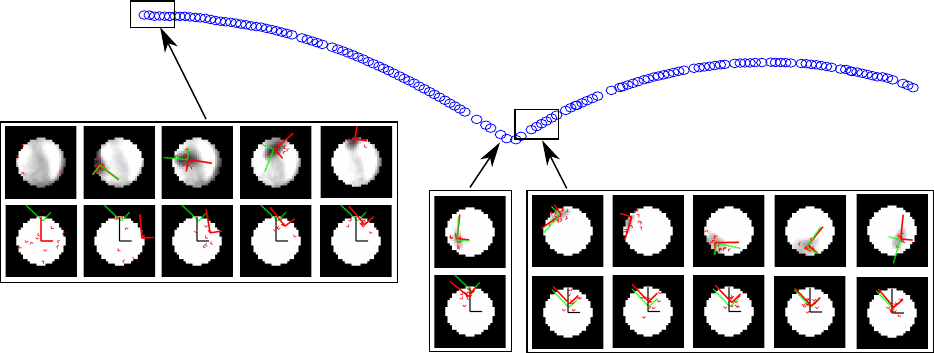
In Figure 8 we show an example of the output of the
second-order QBF we used to track the orientation and
6
Spin was classified into one of the 12 spin types by taking the average
ground truth spin for each spin type and choosing the one with the highest
likelihood with respect to the current spin belief.
−20 −15 −10 −5 0 5 10 15 20
0
0.2
0.4
0.6
time
radians
spin error
QBF−2 + bounce
QBF−2
Fig. 7. Average QBF spin tracking error as it tracks the spin through
the ball’s bounce on the table. Post-bounce errors are significantly lower
with the sample-based bounce tracking method (solid black line) outlined
section V-A.
spin on the ball through one of the underpin/left-sidespin
trajectories. In the first image frame, no logo is detected, so
the orientation distribution is initialized to the “dark side”
of the ball, and the spin distribution is close to a uniform
distribution. After a few more frames, the filter has an
accurate estimate of both the orientation and spin of the ball,
with fairly high concentration parameters (low-uncertainty)
in its Bingham distributions. After the bounce, the sample-
based process update correctly updates the orientation and
spin on the ball, and the filter maintains correct, high-
concentration distributions.
VII. CONCLUSION
For many control and vision applications, the state of a
dynamic process involving 3-D orientations and spins must
be estimated over time, given noisy observations. Previ-
orientations
spins
Fig. 8. An example ball trajectory (underspin + left-sidespin) and the state of the QBF as it tracks the ball’s orientation and spin through the bounce. In
the top row of ball images, the big red (solid-line) axis is the mode of the QBF’s orientation distribution, and the small red axes are random samples from
the orientation distribution. The big green (dashed-line) axis is the detected ball orientation in that image. In the bottom row, the big red (solid-line) axis
is the mode of the QBF’s spin distribution, and the small red axes are random samples from the spin distribution. The big green (dashed-line) axis is the
ground truth spin, and the black axis in the center is the identity (no-spin), for reference.
ously, such estimation was limited to slow-moving signals
with low-noise observations, where linear approximations
to 3-D rotation space were adequate. The contribution of
our approach is that the quaternion Bingham filter encodes
uncertainty directly on the unit quaternion hypersphere,
using a distribution—the Bingham—with nice mathematical
properties enabling efficient approximate inference, with no
restrictions on the magnitude of process dynamics or obser-
vation noise. Because of the compact nature of 3-D rotation
space and the flexibility of the Bingham distribution, we can
use the QBF not only for tracking but also for identification
of signals, by starting the QBF with an extremely unbiased
prior, a feat which previously could only be matched by
more computationally-intensive algorithms, such as discrete
Bayesian filters or particle filters.
REFERENCES
[1] Russell L. Andersson. A robot ping-pong player: experiment in real-
time intelligent control. MIT Press, Cambridge, MA, USA, 1988.
[2] Christopher Bingham. An antipodally symmetric distribution on the
sphere. The Annals of Statistics, 2(6):1201–1225, November 1974.
[3] Xavier Boyen and Daphne Koller. Tractable inference for complex
stochastic processes. In Proceedings of the Fourteenth conference
on Uncertainty in artificial intelligence, UAI’98, page 3342, San
Francisco, CA, USA, 1998. Morgan Kaufmann Publishers Inc.
[4] Yee-Jin Cheon and Jong-Hwan Kim. Unscented filtering in a unit
quaternion space for spacecraft attitude estimation. In Industrial
Electronics, 2007. ISIE 2007. IEEE International Symposium on, pages
66–71, 2007.
[5] D. Choukroun, I.Y. Bar-Itzhack, and Y. Oshman. Novel quaternion
Kalman filter. Aerospace and Electronic Systems, IEEE Transactions
on, 42(1):174–190, 2006.
[6] Wendelin Feiten, Pradeep Atwal, Robert Eidenberger, and Thilo
Grundmann. 6D pose uncertainty in robotic perception. In Advances
in Robotics Research, pages 89–98. Springer Berlin Heidelberg, 2009.
[7] Jared Glover and Leslie Pack Kaelbling. Tracking 3-d rotations with
the quaternion bingham filter. Technical Report MIT-CSAIL-TR-2013-
005, 2013.
[8] Jared Glover and Sanja Popovic. Bingham procrustean alignment for
object detection in clutter. In Proceedings of IEEE/RSJ International
Conference on Intelligent Robots and Systems (IROS), 2013.
[9] Jared Glover, Radu Rusu, and Gary Bradski. Monte carlo pose
estimation with quaternion kernels and the bingham distribution. In
Proceedings of Robotics: Science and Systems, Los Angeles, CA,
USA, June 2011.
[10] A. Kim and M.F. Golnaraghi. A quaternion-based orientation estima-
tion algorithm using an inertial measurement unit. In Position Location
and Navigation Symposium, 2004. PLANS 2004, pages 268–272, 2004.
[11] E. Kraft. A quaternion-based unscented Kalman filter for orientation
tracking. In Information Fusion, 2003. Proceedings of the Sixth
International Conference of, volume 1, pages 47–54, 2003.
[12] Gerhard Kurz, Igor Gilitschenski, Simon Julier, and Uwe D Hanebeck.
Recursive estimation of orientation based on the bingham distribution.
In Information Fusion (FUSION), 2013 16th International Conference
on, pages 1487–1494. IEEE, 2013.
[13] J.J. LaViola. A comparison of unscented and extended Kalman
filtering for estimating quaternion motion. In American Control
Conference, 2003. Proceedings of the 2003, volume 3, pages 2435–
2440 vol.3, 2003.
[14] K. V. Mardia. Characterizations of directional distributions. In
Statistical Distributions in Scientific Work, volume 3, pages 365–385.
D. Reidel Publishing Company, Dordrecht, 1975.
[15] J.L. Marins, Xiaoping Yun, E.R. Bachmann, R.B. McGhee, and M.J.
Zyda. An extended Kalman filter for quaternion-based orientation esti-
mation using MARG sensors. In Intelligent Robots and Systems, 2001.
Proceedings. 2001 IEEE/RSJ International Conference on, volume 4,
pages 2003–2011 vol.4, 2001.
[16] Fumio Miyazaki, Michiya Matsushima, and Masahiro Takeuchi.
Learning to dynamically manipulate: A table tennis robot controls a
ball and rallies with a human being. In Advances in Robot Control,
pages 317–341. 2006.
[17] K. Muelling, J. Kober, O. Kroemer, and J. Peters. Learning to select
and generalize striking movements in robot table tennis. (3):263–279,
2013.
[18] Stephen R Niezgoda and Jared Glover. Unsupervised learning for
efficient texture estimation from limited discrete orientation data.
Metallurgical and Materials Transactions A, pages 1–15, 2013.
[19] S. Schaefer, J. Hakenberg, and J. Warren. Smooth subdivision of
tetrahedral meshes. In Proceedings of the 2004 Eurographics/ACM
SIGGRAPH symposium on Geometry processing, pages 147–154,
Nice, France, 2004. ACM.
[20] Yichao Sun, Rong Xiong, Qiuguo Zhu, Jun Wu, and Jian Chu. Balance
motion generation for a humanoid robot playing table tennis. In
2011 11th IEEE-RAS International Conference on Humanoid Robots
(Humanoids), pages 19–25. IEEE, October 2011.
