The Physics of Juggling a Spinning Ping-Pong Ball.

Portland State University Portland State University

PDXScholar PDXScholar

Physics Faculty Publications and Presentations Physics

10-2016

The Physics of Juggling a Spinning Ping-Pong Ball. The Physics of Juggling a Spinning Ping-Pong Ball.

Ralf Widenhorn

Portland State University

Follow this and additional works at: https://pdxscholar.library.pdx.edu/phy_fac

Part of the Physics Commons

Let us know how access to this document bene;ts you.

Citation Details Citation Details

Widenhorn, R. (2016). The physics of juggling a spinning ping-pong ball. American Journal of Physics,

84(12), 936-942.

This Article is brought to you for free and open access. It has been accepted for inclusion in Physics Faculty

Publications and Presentations by an authorized administrator of PDXScholar. Please contact us if we can make

this document more accessible: [email protected].

The physics of juggling a spinning ping-pong ball

Ralf Widenhorn

Department of Physics, Portland State University, Portland, Oregon 97201

(Received 14 August 2015; accepted 18 September 2016)

Juggling a spinning ball with a ping-pong paddle represents a challenge both in terms of hand-eye

coordination and physics concepts. Here, we analyze the ping-pong ball’s motion, and explore how

the correct paddle angle relates to the ball’s spin and speed, as it moves vertically up and down. For

students, this requires engaging with concepts like momentum, angular momentum, free-body

diagrams, and friction. The activities described in this article include high-speed video motion

tracking of the ping-pong ball and the investigation of the frictional characteristics of the paddle. They

can be done in a physics lab or at home, requiring only inexpensive or commonly used equipment,

and can be undertaken by high school or college students.

2016 American Association of Physics Teachers.

[http://dx.doi.org/10.1119/1.4964104]

I. INTRODUCTION

Students usually get their ﬁrst introduction to physics

through mechanics. The study of motion provides various

opportunities for lab activities. Although students have devel-

oped an intuition through everyday experience of how objects

move, the challenges for students to correctly understand these

concepts have been well documented since the early years

of physics education research.

While a standard laboratory

experiment aims to teach important concepts and experimental

skills, we ﬁnd few “typical” experiments excite our students.

Furthermore, labs frequently suffer from being “cookbook

style,” with little room for students to actively engage and

explore physics phenomena, or to develop true experimental

skills that have been identiﬁed as important by the American

Association of Physics Teachers Recommendations for the

Undergraduate Physics Laboratory Curriculum

and the Next

Generation Science Standards.

One way to allow students to

more freely explore basic physics principles and develop

experimental skills is to have them work on a project lab.

good project leaves room for students to explore different

aspects of a phenomenon, is challenging, captures a student’s

interest, and at the same time provides the opportunity to dis-

cuss experimental design.

The exploration of physics phenomena in sports can pro-

vide an extra stimulus to spark the interest of many students

and has been the subject of several textbooks.

5,6

However, it

is difﬁcult to investigate sports activities in a lab environ-

ment. Table tennis, often referred to colloquially as ping-

pong, uses a light ball that can be easily studied in a conﬁned

space. A key difference between competitive table tennis

and recreational ping-pong is the use of spin. The spin of a

ping-pong ball is difﬁcult to observe directly, but its effect

on all aspects of the game is profound. The mass of the ball

is small and the ball’s trajectory and its motion upon bounc-

ing off the table and paddle are non-intuitive for all but the

most experienced players (see Fig. 1). While this makes it

more difﬁcult to predict a ball’s trajectory, it also makes the

motion more intriguing to analyze. Concepts like kinematics,

projectile motion, free-body diagrams, friction, air resis-

tance, the Magnus force, kinetic energy, rotational kinetic

energy, impulse, forces, and angular momentum can all play

an important role in such an analysis. Various articles have

been written on the bounce of spinning balls in ping-

pong

7–12

and other types of spinning balls upon hitting a rac-

quet, paddle, club, or the ground.

13–25

Following up on these

studies, we present a project that many students who enjoy

ball sports will ﬁnd to be a challenge to their hand-eye coor-

dination and their physics skills. For our study we will focus

on the effect of spin on the bounce of the ping-pong ball.

Due to the relatively small speeds involved we will neglect

drag forces

26–28

and the curving of the ball due to the

Magnus force.

29–33

The goal here is to hit a ping-pong ball upward with some

spin, and try to control it when it impacts the paddle to send

it straight up again, so that it can easily be caught afterwards.

Such an exercise helps a player to get a feel for the speed

and tackiness of the paddle. For the study described in this

manuscript, we use a standard 40-mm plastic ping-pong ball

with a pre-assembled entry level Stiga Inspire paddle with

Magic rubber (1.5-mm sponge)

and the competitive grade

combo of a Butterﬂy Tenergy 05 rubber (2.1-mm sponge)

on a Timo Boll Spirit blade.

The lower quality Magic rub-

ber had lost its initial tackiness while the Tenergy rubber

was still tacky.

One can send a ball without spin straight up, by placing

the paddle ﬂat under the ball, but in the case of a spinning

ball the paddle needs to be angled as shown in Fig. 2. With

some practice, one can develop a good intuition on how to

angle the paddle and juggle the spinning ball multiple times

by alternating the angle of the paddle from being titled

clockwise to counterclockwise, sending the ball straight up

each time. To analyze this motion a couple of research ques-

tions might include: “At what angle a, does the paddle need

to be placed to have the ball go vertically upward for differ-

ent initial and ﬁnal speeds and spins of the ball?” and “How

does this angle depend on the type of paddle?”

II. MOTION TRACKING

We used a point-and-shoot Casio Exilim EX-FH100

camera

that captures video in the high frame rate shooting

modes of 240 fps at 448  336 pixels, and at 1,000 fps at

224  64 pixels. The compact consumer camera was equipped

with an SD card rated for 10MB/s and was mounted on a stan-

dard tripod. We use Vernier Logger Pro software to extract

data from the videos using frame-by-frame tracking of the

ball.

For students new to ping-pong, the ﬁrst step is to practice

how to brush the ping-pong ball from underneath with the

paddle such that the ball has a large spin and ﬂies up approx-

imately vertically. Next, students will record their attempts

936 Am. J. Phys. 84 (12), December 2016 http://aapt.org/ajp

2016 American Association of Physics Teachers 936

to hold the paddle such that the ball pops straight up, catch-

ing the ball after each try. Even though it is a fun challenge,

one does not need to juggle the ball multiple times for this

project. For the video capture, it is easiest to use a tripod so

that one can easily adjust the level and angle of the camera.

For the study described in this section, we chose a frame rate

of 240 fps, which provides sufﬁcient spatial resolution for

motion tracking. One ﬁnds that the ball velocities for this

experiment are on the order of a few meters per second or

less and are easily tracked at a lower frame rate. However,

the spin can be such that a high frame rate is required to

track the rotational speed of the ball. The 240 fps frame rate

would have a ball spinning at 60 rev/s rotate by an easily

traceable quarter of revolution from frame to frame.

Particularly for students interested in engineering, this would

be a good opportunity to explore signal processing, the

Nyquist frequency, and aliasing effects. Drawing a black line

around the circumference of the ball and adding two dots at

the ball’s polar opposites allowed the ability to track the

ball’s spin. The rotational velocity is found by counting the

rotations of the line or dots from frame to frame. Video

acquisition should be done in a well-lit room, avoiding

incandescence and other light sources that exhibit power line

ﬂicker.

Figure 1 shows the impact of the spin on the bounce of the

ball. The ball rotated counterclockwise (from the perspective

of the reader) three times over 36 frames before bouncing

off the paddle. Deﬁning a clockwise rotation as positive,

the angular velocity of the spinning ball was therefore x

¼240 fps=ð12 f=revÞ¼20 rev=s. Following the bounce,

the ball rotated clockwise once over 38 frames, resulting in

an angular velocity of x

¼ 6:3 rev=s.

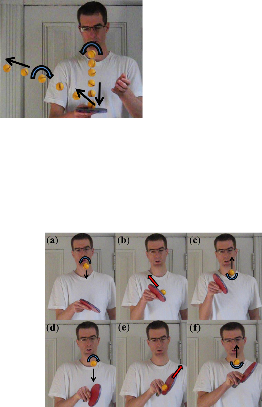
To prevent the ball from bouncing off to the side, one

needs to angle the paddle. The counterclockwise rotation of

the ball before impact, as shown in Fig. 2(a), requires

angling the paddle as depicted in Fig. 2(b). Moving the pad-

dle as indicated with the arrows in Figs. 2(b) and 2(e) will

add extra speed and counter-rotation to the ball. Upon

impact, the ball rises and then falls, as shown in Figs. 2(c)

and 2(d) while now spinning clockwise. A ball with this spin

would jump to the right if the paddle is held horizontally,

hence the paddle needs to be angled as shown in Fig. 2(d).

Fig. 1. Overlay image of a spinning ball dropping vertically onto a horizon-

tal paddle. The video was taken at a frame rate of 240 fps, and the ball loca-

tion is shown for every tenth frame, approximately 41.7 ms apart.

Fig. 2. Sequence of images when juggling a spinning ping-pong ball. The frames were selected to illustrate one complete juggling cycle: (a) ball falling verti-

cally and rotating counterclockwise; (b) angled paddle impacting the ball, the paddle moves in the direction as indicated by the arrow; (c) ball moving verti-

cally upwards after impact while rotating clockwise; (d) ball dropping back vertically toward the paddle while still rotating clockwise; (e) angled paddle

impacting the ball, the paddle moves in the direction as indicated by the arrow; (f) ball moving vertically upward after impact while rotating counterclockwise.

937 Am. J. Phys., Vol. 84, No. 12, December 2016 Ralf Widenhorn 937

After impact, the ball will move upwards with a counter-

clockwise spin as shown in Fig. 2(e). A skilled student can

repeat the sequence as the ball falls again, as in Fig. 2(a). For

the motion analysis, it is sufﬁcient to consider the ﬁrst three

ﬁgures as the paddle angle and ball motion of the following

part of the sequence are symmetric with rotational directions

and the horizontal axis ﬂipped.

To convert the pixel distance in the frame-by-frame track-

ing of the ball to a physical distance, one needs to calibrate it

with an object of known length. The calibration was done by

displaying a 50-cm ruler in the plane of motion at one point

during the video capture. With this reference distance and

the frame rate of the video capture, one can plot horizontal

and vertical distances and velocities as a function of time.

For this study, the camera was about 3 m away from the ball,

resulting in small angles for the vertical positions analyzed.

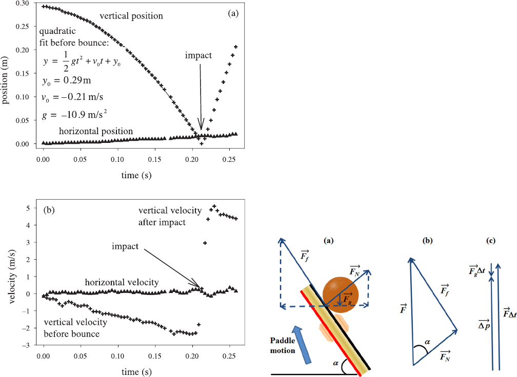
Figure 3(a) shows the position during the fall of a ball

from close to its peak motion to after it hits the paddle. The

ball drops and rises almost vertically with a slight movement

to the right throughout its trajectory. The vertical position

before impact varies quadratically as a function of time. The

best-ﬁt line results in a gravitational acceleration slightly

larger than the theoretical value, pointing to the calibration

length being slightly off. This can be due the fact that the

height of the exact contact point with the ball, and the height

from which the ball dropped, varied from trial to trial and

therefore is not always in line with the position of the ruler

during calibration. The exact distance of the plane of motion

of the ball from the camera varied from trial to trial as

well. Each point on the velocity versus time graph shown in

Fig. 3(b) is calculated from a seven frames kernel to calcu-

late the derivative of the position data in Fig. 3(a). This

causes the smoothing of the velocity data, which is espe-

cially visible for v

around the point of impact.

The data shown in Fig. 3 indicate that the horizontal

velocity was small throughout the motion, and the ball suc-

cessfully bounces almost vertically off the paddle. Under the

inﬂuence of gravity, the magnitude of the vertical velocity

increases linearly with time until the ball hits the paddle and

changes direction. The large magnitude of the velocity after

impact indicates that the paddle added extra translational

kinetic energy to the ball. The velocity v

before and the

velocity v

after impact can be obtained from linear ﬁts to the

corresponding data points. The data points for the three

frames before and after the bounce are not accurate, due to

the smoothing of the velocity data and are not included in

the ﬁts. The small changes in the horizontal velocity further

indicate that the speed of the ball is small enough so that the

Magnus force did not have a signiﬁcant impact on the

trajectory.

III. MOTION ANALYSIS

To analyze the motion of the ball, one needs to consider

both its spin and linear velocity. Figure 4(a) shows all forces

acting on the ball on impact. The weight of the ball is

included for pedagogical reasons though for most cases it

will be small compared to the other forces during impact.

Choosing the center of the ping-pong ball as the rotational

axis, we can calculate the change in angular momentum by

multiplying the torque s by the time over which it acts Dt,

giving

DL ¼ sDt ¼ F

rDt ¼ FrDt sin a; (1)

where r is the radius of the ball (see Fig. 4 for the deﬁnitions

of F

, F, and a). Meanwhile, the change in linear momentum

in the vertical direction is

Dp ¼ FDt  F

Dt; (2)

which can be expressed as

Fig. 3. (a) Frame-by-frame position tracking of the ball in the horizontal and

vertical directions. (b) Corresponding horizontal and vertical velocities as a

function of time.

Fig. 4. (a) Forces acting on the ball as it bounces off the paddle upon impact.

(b) The vector sum of the frictional force F

and the normal force F

result in a

vertical net force on the ball. (c) Impulse and change in momentum of the ball.

938 Am. J. Phys., Vol. 84, No. 12, December 2016 Ralf Widenhorn 938

F ¼

þ F

: (3)

Inserting Eq. (3) into Eq. (1) then gives

DL ¼

þ F



rDt sin a; (4)

and solving for a results in

sin a ¼

rDt Dp=Dt þ F



: (5)

Since the weight of the ping-pong ball is small and in most

cases

Dp=Dt  F

; (6)

this result becomes

sin a ¼

rDp

: (7)

We note that in vector notation this equation can be

expressed simply as D

L ¼

r  D

p. To ﬁnd the angle a in

terms of the measurable quantities Dx and Dv, we need to

replace Dp and DL in Eq. (7). Though one could include the

thickness of the ping-ping ball shell,

39,40

we are assuming

the ping-pong ball has the moment of inertia of a hollow

sphere so the change in angular momentum can be calculated

using

I ¼

; (8)

giving

DL ¼ I x

 x

ðÞ

Dx: (9)

Using

Dp ¼ mð v

 v

Þ¼mDv (10)

and inserting Eqs. (9) and (10) into Eq. (7) results in

sin a ¼

2rDx

3Dv

: (11)

The minimum required coefﬁcient of friction of the rubber

sheet at the angle a can then be calculated (see Fig. 4) from

min

¼ tan a: (12)

Table I shows a set of data taken with both paddles. Trials 1

and 2 attempted to move the paddle very little on impact and

still have the ball bounce upward. One can observe that for

both paddles, the ball bounces off with a slightly smaller

speed. The elastic Tenergy rubber sheet reverses the spin

almost completely. Other trials, with little movement of the

paddle, showed x

is generally slightly smaller than x

, but

overall conﬁrmed that most of the spin is inverted and there-

fore has a large tangential coefﬁcient of restitution (ratio of the

outgoing and incoming velocity tangential to the ball surface)

for this rubber sheet. For the Magic rubber, there is almost no

spin after the bounce. It was generally found that little paddle

movement resulted in a small inverted spin corresponding to a

tangential coefﬁcient of restitution of close to zero for this rub-

ber sheet. The angle a is calculated using Eq. (11) and com-

pared with a

measured

, which is determined by measuring the

physical placement of the paddle in the frame of impact using

a virtual ruler in Logger Pro.

If we want to send a ball with x

and v

vertically upwards

to the same level, with little movement of the paddle, we can

determine the angle at which to place the paddle: Dv needs to

be equal to 2v

to reach the same level. For the Tenergy rub-

ber, we can approximate Dx ¼ 2x

and Eq. (11) results in

sin a ¼

2rx

: (13)

Meanwhile, in a ﬁrst approximation, the ball loses most of

its rotation upon impact for the Magic rubber sheet.

Assuming x

¼ 0 Eq. (11) leads to

sin a ¼

: (14)

Sending the ball back to the same level with little movement

of the paddle therefore requires angling the tacky and elastic

Tenergy rubber paddle at a larger angle than the paddle with

the Magic rubber. For the Tenergy paddle, the rotation is

inverted and one could juggle a ball as often as one likes up

and down by alternating the paddle angle from þa to a.

The Magic rubber causes the ball to lose most of its spin,

and one could place the paddle almost horizontally on the

next stroke.

For both paddles, we can vary the spin and velocity of the

ball by striking it with a greater paddle speed. Depending on

the direction of the paddle motion, one imparts more spin or

translational velocity on the ball. As long as Eq. (11) is satis-

ﬁed, the ball will travel straight up. By increasing the spin,

one increases the change in angular momentum and hence

the paddle angle. Trials 3 and 4 both increase the spin and

translational velocity. A large change in the angular velocity,

as in trial 4, will result in a more angled paddle. Trial 5 is an

example of a slow ball being sent back to roughly the same

level with a slight increase in rotational kinetic energy and a

strongly angled paddle. Trial 6 shows that one can invert the

spin with the Magic rubber paddle, however, this requires

moving the paddle quickly in the direction of the angle a.

The result for the Magic rubber demonstrates that one can

continuously juggle the ball if one adds a signiﬁcant swing

Table I. Paddle angle for different vertical and angular velocities. The quan-

tities x

, x

, v

, and v

are determined from motion tracking, a

measured

is found

from position measurements on the frame of impact, a is calculated using

Eq. (11), and l

min

is found from Eq. (12).

Trial Rubber

(rev/s)

(m/s)

(deg)

measured

(deg)

diff.

min

¼ tan a

1 Tenergy 17 17 3.7 3.2 24 20 16 0.44

2 Magic 18 2 2.4 2.2 20 19 8 0.37

3 Tenergy 12 37 3.2 4.1 34 34 0 0.67

4 Tenergy 28 41 2.4 5 51 52 2 1.22

5 Tenergy 18 25 2.1 2.2 54 45 17 1.37

6 Magic 12 11 2.1 2.6 25 24



3 0.46

939 Am. J. Phys., Vol. 84, No. 12, December 2016 Ralf Widenhorn 939

of the paddle. Thus, even though the paddle angle for the

Magic and Tenergy rubber would be identical for the same

Dx and Dv, the motion of the paddle would be quite differ-

ent. The necessary fast swing of the Magic paddle along the

direction of a makes juggling the ball with the Magic paddle

more difﬁcult and requires more effort by the player than

with the Tenergy paddle where a slow motion at the correct

angle is sufﬁcient.

Note that in Table I, the experimental difference between

the measured and calculated angles is largest for trials 1 and

5. In both of these cases a is larger than a

measured

. A larger a

corresponds to a larger change in the horizontal velocity and

for these two trials the trajectory was the least vertical, with

a horizontal velocity change of 0.3–0.5 m/s. The impact of

the earlier mentioned slight calibration error appears to be

minor, but being successful in getting the ball going straight

up and down impacts the agreement of theory and experi-

mental data more strongly. We think the data presented here

are what one can reasonably expect from students, though

some dedicated students with great hand-eye coordination

may be able to get a lower experimental difference.

Equation (11) restricts all solutions to Dx < 3Dv=2r.

However, while all possible solutions must satisfy Eq. (11),

for large angles the normal force decreases and the required

frictional force may exceed the maximum friction that can be

supplied by the paddle rubber. Hence, Eq. (11) is a necessary

but not sufﬁcient condition. We will try in Secs. IV and V to

estimate the required coefﬁcient of friction of the rubber sheet

necessary to exert a large enough frictional force.

IV. TIME OF CONTACT

To observe the impact of the ball, we set the frame rate to

1,000 fps. The camera was placed right next to the paddle

and captured the impact of a ball dropped with little spin

from a height of 0.5–1 m with the paddle placed horizontally

and angled at 45



. We found that the impact for both paddle

angles showed similar results at this temporal resolution.

The high frame rate, and therefore short integration times,

required good lighting conditions.

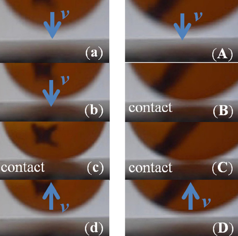
The images in Fig. 5 were taken using natural sunlight and

the Butterﬂy paddle placed horizontally. From the video

images, using the size of the ball as a reference, one can esti-

mate the distance of the ball from the paddle. From these dis-

tances and the inspection of the images close to impact, one

can get a rough estimate of the contact time. Of the eight

drops we looked at, two showed contact in only one frame

(like the left sequence in Fig. 5), while two trials showed

contact in two frames (like the right sequence in Fig. 5). The

other four trials had one frame with clear contact and another

frame so close that the ball may or may not have been in

contact with the paddle. The fact that there were trials with

only a single image showing full contact places an upper

limit for the contact time at 2 ms. The trials showing two

sequential images with contact place a lower limit for the

contact time at 1 ms. For contact times of 1–2 ms and typical

changes in speed of 4–8 m/s, Dp=Dt for the 2.7-g ping-pong

ball is in the range of approximately 5–20 N, at least two

orders of magnitude larger than F

, thus satisfying the condi-

tion that Dp=Dt  F

. The slight downward impulse due to

gravity shown in Fig. 4(c) is therefore indeed negligible. We

can calculate the normal force on the ping-pong ball as

¼ðDp=DtÞ cos a, and knowing the order of magnitude of

the forces during contact with the paddle, we can investigate

the frictional forces supplied by the paddle.

V. FRICTION

The normal force exerted on the ball by the paddle varies

quickly during impact. For this study, we did not obtain time

resolved force versus time data and we need to make some

simplifying assumptions. We ignore any dependence of the

contact time on the paddle angle, speed, and type, as well as

the speed and spin of the ball. With the rough estimate of

contact time, we can estimate normal and frictional forces if

we know the coefﬁcient of friction of the rubber sheet.

For this, we conducted a classical friction experiment by

sliding the ping-pong ball, with different weights added,

across the surface of interest (the rubber sheet). Figure 6

shows the experimental setup. The ping-pong ball was placed

in a measuring cup and ﬁxed with masking tape so that it

could not rotate. The total mass of the tape, ball, and measur-

ing cup was 61 g. A 50-g weight hanger is attached for all but

the measurement with the lowest normal force. Additional

masses, up to a total of 1,511 g, are added in 100-g incre-

ments. The weight hanger is stabilized with minimal vertical

force with one hand while the other hand applies a horizontal

force that is measured with a force sensor. The force is

increased until the ball starts to slide for a short distance of

1–3 cm, and this is repeated at least six times. The average

and standard deviation of the peak force of six measurements

is calculated and plotted as a function of the normal force in

Fig. 7(a).

For many surfaces, the maximum frictional force increases

linearly with the normal force, with the coefﬁcient of friction

l as the constant of proportionality. However, the elastic

rubber sheet has a coefﬁcient of friction that depends on the

normal force.

The normal-force-dependent frictional

Fig. 5. High speed capture (1,000 fps) of two drops on the Tenergy paddle.

The ball had little spin and both the paddle and camera were angled horizon-

tally. The images are sequential starting with frames (a/A) and ending with

frames (d/D) with 1 ms between frames. The ball is in contact with the pad-

dle in frame (c) on the left and in frames (B) and (C) on the right.

940 Am. J. Phys., Vol. 84, No. 12, December 2016 Ralf Widenhorn 940

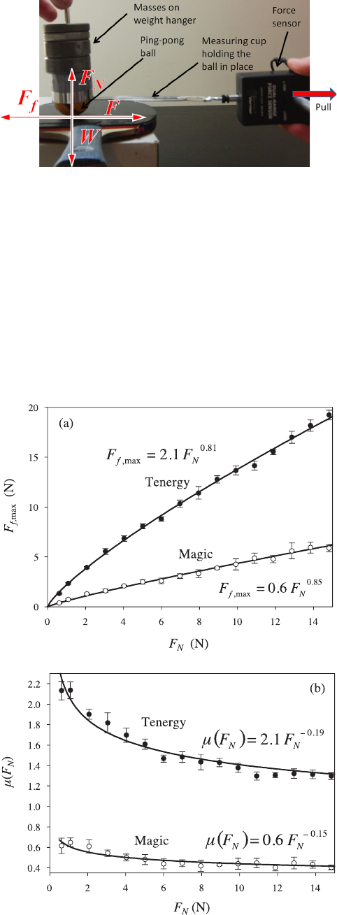
coefﬁcient is calculated as the ratio F

and is plotted in

Fig. 7(b). The data for both rubber sheets can be ﬁtted empir-

ically with a power law of the form

lðF

Þ¼2:1F

0:19

ðTenergyÞ; (15)

and

lðF

Þ¼0:6F

0:15

ðMagicÞ; (16)

where F

is measured in Newtons. For example, for a small

normal force of 1 N the frictional coefﬁcient for the Tenergy

is 2.1, answering the classic physics classroom question if l

can be larger than one. The Tenergy coefﬁcient of friction

decreases for larger normal forces to about 1.3 at F

¼ 15 N.

For the same normal forces, the Magic rubber sheet has a

coefﬁcient of friction of about 0.6 and 0.4, respectively.

The last column in Table I shows that for trials 1 and 3 the

actual coefﬁcient of friction of the Tenergy rubber vastly

exceeds the l

min

values of 0.44 and 0.67. Because of the larger

angle of the Tenergy paddle for trials 4 and 5, the required

min

values of 1.22 and 1.37 are much closer to the actual fric-

tional coefﬁcient. Meanwhile, for both trials with the Magic

rubber, the coefﬁcients of friction are such that l

min

is on the

orderoftheactuall. The small maximum frictional force is

barely sufﬁcient even for the small angles in these trials, which

is reﬂected in practice by the difﬁculty of juggling the ball

with large paddle angles for the Magic rubber. On the other

hand, the larger frictional coefﬁcient of the Tenergy paddle

gives it the feel of more control even for larger angles. The

largest paddle angles can be obtained for a combination of

small Dx; Dv pairs, taking advantage of the higher coefﬁcient

of friction for small normal forces. To accomplish this, one

would need to brush the ball close to the top of its trajectory at

a large angle; this would give the ball a small velocity change,

effectively juggling the ball almost in place.

VI. CONCLUSION

We demonstrated that one can investigate the juggling of a

spinning ping-pong ball with different paddles using basic

concepts from high school or college level introductory phys-

ics and inexpensive and commonly available lab equipment.

A study like this would be an ideal project for students who

enjoy ball sports. Further studies could include the investiga-

tion of contact time, coefﬁcients of restitution, and force, with

higher temporal resolution for different speeds, angles, spins,

paddles, and balls. Moreover, motion analysis could be used

to explore how the speed and direction of the paddle motion

during impact with the ball inﬂuences the change in linear and

angular velocities. The activities described here are both well-

deﬁned and rich in interesting open-ended research questions.

The measurements require both experimental skill and appli-

cation of physics that spans most concepts of mechanics in a

way that we hope will be engaging to many students.

ACKNOWLEDGMENTS

The author wants to acknowledge Grace Van Ness,

Michael Fitzgibbons, Pure Pong in the Pearl, and the

anonymous reviewers for their support and helpful feedback.

Electronic mail: [email protected]

D. Hestenes, M. Wells, and G. Swackhamer, “Force concept inventory,”

Phys. Teach. 30, 141–158 (1992).

AAPT Recommendations for the Undergraduate Physics Laboratory

Curriculum <https://www.aapt.org/Resources/upload/LabGuidlines

Document_EBendorsed_nov10.pdf> (accessed November 19, 2015).

Next Generation Science Standards <http://www.nextgenscience.org/>

(accessed June 18, 2016).

P. Gluck and J. King, Physics Project Lab (Oxford U.P., UK, 2015);

available at https://www.amazon.com/Physics-Project-Lab-Paul-Gluck/dp/

0198704585 and http://global.oup.com/about/?cc=us.

V. McInnes Spathopoulos, An Introduction to the Physics of Sports

(Independent Publishing Platform, 2013) available at https://

Fig. 6. Setup and free-body diagram for the measurement of the maximum

frictional force for different normal forces.

Fig. 7. (a) Maximum frictional force of the Tenergy and Magic rubber sheets

for different normal forces. (b) Ratio of the maximum frictional force F

f ;max

to the normal force F

versus normal force; this ratio represents the effective

coefﬁcient of friction for a particular normal force.

941 Am. J. Phys., Vol. 84, No. 12, December 2016 Ralf Widenhorn 941

www.amazon.com/Introduction-Physics-Vassilios-McInnes-Spathopoulos/

dp/1483930076 and https://www.createspace.com/.

M. A. Lisa, The Physics of Sports (McGraw-Hill Higher Education,

Columbus, OH, 2015); available at https://www.amazon.com/Physics-

Sports-Michael-Lisa/dp/0073513970 and http://www.mheducation.com/.

A. Nakashima, Y. Ogawa, Y. Kobayashi, and Y. Hayakawa, “Modeling

of rebound phenomenon of a rigid ball with friction and elastic effects,”

Proceedings of IEEE American. Control Conference (2010), pp.

1410–1415.

S. Araki, S. Sato, and H. Yamazaki, “Collisional properties of ball-racket

interactions in terms of normal and tangential coefﬁcients of restitution,”

Int. J. Table Tennis Sci. 3, 17–49 (1996).

L. Pauchard and S. Rica, “Contact and compression of elastic spherical

shells: the physics of a ping-pong ball,” Philos. Mag. B 78(2), 225–233

(1998).

K. Tiefenbacher and A. Durey, “The impact of the table tennis ball on the

racket (backside coverings),” Int. J. Table Tennis Sci. 2, 1–14 (1994).

C. M. Graney, “Taking a swat at physics with a ping-pong paddle,” Phys.

Teach. 32, 94–98 (1994).

K. Kamijima, Y. Ushiyama, T. Yasaka, and M. Ooba, “Effect of different

playing surfaces of the table on ball bounces in table tennis,” The 13th

ITTF Sports Science Congress May 11-12, Paris, France (2013), pp.

53–56.

R. B. Clark, “That’s the way the bouncing ball spins,” Phys. Teach. 44,

550–551 (2006).

P. Knipp, “Bouncing balls that spin,” Phys. Teach. 46, 95–96 (2008).

A. Domnech, “A classical experiment revisited: The bounce of balls and

superballs in three dimensions,” Am. J. Phys. 73, 28–36 (2005).

R. Cross, “Enhancing the bounce of a ball,” Phys. Teach. 48, 450–452

(2010).

R. Cross, “The bounce of a ball,” Am. J. Phys. 67, 222–227 (1999).

R. Cross, “Grip-slip behavior of a bouncing ball,” Am. J. Phys. 70,

1093–1102 (2002).

R. Cross, “Measurements of the horizontal coefﬁcient of restitution for a

superball and a tennis ball,” Am. J. Phys. 70, 482–489 (2002).

R. Cross, “Impact of a ball with a bat or racket,” Am. J. Phys. 67, 692–702

(1999).

R. Cross, “The coefﬁcient of restitution for collisions of happy balls,

unhappy balls, and tennis balls,” Am.J.Phys.68, 1025–1031

(2000).

R. Cross, “Bounce of a spinning ball near normal incidence,” Am. J. Phys.

73, 914–920 (2005).

W. A. Turner and G. W. Ellis, “The energetics of a bouncing ball,” Phys.

Teach. 37, 496–498 (1999).

H. Brody, “That’s how the ball bounces,” Phys. Teach. 22, 494–497

(1984).

P. A. Maurone and F. J. Wunderlich, “Bouncing ball experiment,” Am. J.

Phys. 46, 413–415 (1978).

M. Nagurka, “Aerodynamic effects in a dropped ping-pong ball

experiment,” Int. J. Eng. Educ. 19(4), 623–630 (2003).

M. E. Brandan, M. Guti



errez, R. Labb



e, and A. Menchaca-Rocha,

“Measurement of the terminal velocity in air of a ping pong ball using a

time to amplitude converter in the millisecond range,” Am. J. Phys. 52,

890–893 (1984).

R. M. French, “Part 4: Dropping a ping-pong ball,” Exp. Tech. 30(2),

59–60 (2006).

C. Clanet, “Sports ballistics,” Annu. Rev. Fluid Mech. 47, 455–478 (2015).

F. Yamamoto, Y. Tsuji, G. Chen, M. Ogawa, and M. Nakagawa, “Basic

theory and experiment for the simulation of ball trajectory,” Int. J. Table

Tennis Sci. 3, 1–15 (1996).

F. Yamamoto, J. Kasai, H. Hirakawa, S. Someya, and K. Okamoto, “High-

speed video image analysis of air ﬂow around a table tennis ball,” Int. J.

Table Tennis Sci. 6, 149–150 (2010).

K. Ou, P. Castonguay, and A. Jameson, “Computational sports aerodynam-

ics of a moving sphere: Simulating a ping pong ball in free ﬂight,” in 29th

AIAA Applied Aerodynamics Conference (2011), pp. 1–16.

Y. Huang, D. Xu, M. Tan, and H. Su, “Trajectory prediction of spinning

ball for ping-pong player robot,” IEEE/RSJ International Conference on

Intelligent Robots and Systems (2011), pp. 3434–3439.

More information on the Stiga Inspire can be found at <http://stigatable-

tennis.com/en/products/inspire/> (accessed June 18, 2016).

More information on Tenergy rubber can be found at <http://shop.butter-

ﬂyonline.com/tenergy-05> (accessed June 18, 2016).

More information on the Timo Boll Spirit blade can be found at <http://

shop.butterﬂyonline.com/timo-boll-spirit> (accessed June 18, 2016).

More information on the Casio EX-FH100 can be found at <http://

www.casio-intl.com/asia-mea/en/dc/ex_fh100/> (accessed June 18, 2016).

More information about Logger Pro can be found at <http://www.vernier.-

com/products/software/lp/> (accessed November 19, 2015).

X. Cao, “Moment of inertia of a ping-pong ball,” Phys. Teach. 50, 292

(2012).

J. Mallinckrodt, “Errant ping-pong ball,” Phys. Teach. 50, 389 (2012).

A. Schallamach, “The load dependence of rubber friction,” Proc. Phys.

Soc. B 65, 657–661 (1952).

942 Am. J. Phys., Vol. 84, No. 12, December 2016 Ralf Widenhorn 942